Machine learning systems
Attention Is All You Need
The big idea
A machine-learning model cannot read a sentence as humans do. It receives numbers and must learn which numbers are related. Before Transformers, many sequence models read text one item at a time and carried a running memory forward. This worked, but made long-range relationships and parallel computation difficult.
A Transformer starts from a different idea: let each token directly inspect every other relevant token. The mechanism that decides what to inspect is called attention. Attention does not replace the rest of a neural network; it is the information-routing operation at the center of each Transformer block.
We will carry one sentence through the complete architecture: Ninja moved the plant near the window because it needed more sunlight. This example makes attention useful immediately: the model must connect it to plant, not to the closer noun window. The vectors are deliberately tiny so every calculation remains visible. Real models use the same operations with much larger vectors, more attention heads, and many repeated layers.
Four pieces of math you need
- Scalar
- One number, such as an attention score of 1.4.
- Vector
- A list of numbers describing one token.
- Dot product
- Multiply matching vector entries, then add the results.
- Matrix
- A learnable table that transforms one vector into another.
Experiment in Playground 1: move one stage at a time from tokenization to decoding. First learn the route; the next playgrounds will open each stage and show its numbers.
Source: Vaswani et al., Attention Is All You Need.
Playground 1
Follow One Sentence End To End
Move through the entire Transformer path. Every later playground opens one of these stages and exposes its calculation.
Tokenize
Split text into model vocabulary pieces and map each piece to an ID.
[742, 3812, 101, 2487, 209, 101, 5124, 173, 340, 7281, 430, 9650, 9]1. Text must become numbers
The model first uses a tokenizer. A token may be a word, part of a word, punctuation, or another vocabulary unit. The tokenizer turns each token into an integer ID. That ID is only an address; a larger ID does not mean a more important word.
The ID selects one row from a learned embedding table. If the table is named E, then x_i = E[token_id_i] means: “look up the starting vector for token i.” The vector has d_model numbers. During training, the model adjusts these numbers so tokens useful in similar contexts develop useful geometric relationships.
Our vector for plant has four dimensions, such as[0.80, 0.50, 0.20, 0.60]. Those four entries do not have simple human labels. Together they form a learned representation.
Experiment in Playground 2: select every token. Notice that each vocabulary ID retrieves a different vector, while every vector has the same width. Compare plant and window; focus on the full pattern, not one number.
Playground 2
Token IDs Become Learned Vectors
Select a token to inspect its vocabulary ID and toy embedding. In a real model, this vector has hundreds or thousands of dimensions.
Lookup formula: x_i = E[token_id_i], where E is learned during training. Tokenization decides the IDs; the embedding table supplies the starting geometry.
2. The model also needs word order
Self-attention can compare a collection of vectors, but by itself it does not know which token was first. “Ninja moved the plant near the window” and “The plant moved Ninja near the window” contain similar tokens but express different ideas. A position signal must therefore be combined with each token embedding.
The original Transformer used sine and cosine waves. Each vector dimension oscillates at a different frequency. For an even dimension, the value is a sine; for an odd dimension, it is a cosine. You do not need to memorize the exponent. The important idea is that each position receives a distinctive, smoothly changing numerical signature.
The final input is simply token embedding + positional encoding. Because it is addition, the vector keeps token information while also carrying order information.
Experiment in Playground 3: move the position from 0 to 12. Watch fast-changing dimensions and slow-changing dimensions. Compare neighboring positions, then compare positions far apart.
Playground 3
Position Has To Be Added Back
Move the token position and watch the sinusoidal signature change across dimensions. Even dimensions use sine; odd dimensions use cosine.
PE(pos, 2i) = sin(pos / 10000^(2i/d_model))PE(pos, 2i+1) = cos(pos / 10000^(2i/d_model))Nearby positions produce related signatures. Different dimensions oscillate at different frequencies, making both short and long distances available to later layers.
3. Query, key, and value are three views of a token
Attention gives each token three jobs. A query says what information this token is looking for. A keysays what kind of information this token can match. A value carries the information that will actually be returned.
Think of a search system: the query is what you typed, keys are the searchable labels, and values are the documents returned. A token creates all three using learned matrices:Q = XW_Q, K = XW_K, andV = XW_V.
Multiplying by a matrix means each output number becomes a weighted combination of the input numbers. The three matrices learn different combinations, so Q, K, and V are different even though they start from the same token vector.
Experiment in Playground 4: select one token and compare its input, Q, K, and V vectors. Then change the token. Notice that the projection rule stays fixed while the resulting vectors change with the input.
Playground 4
One Vector, Three Learned Views
Query, key, and value are not copies. Three learned matrices project the same token representation into three different roles.
Query describes what this position seeks. Keydescribes how another position can be matched. Valuecarries the information returned when that match receives weight.
4. Attention measures compatibility
To decide whether one token should read another, the model compares a query with a key using a dot product. Suppose the vectors are [2, 1] and [3, 4]. Their dot product is (2 x 3) + (1 x 4) = 10. Similar directions tend to produce larger scores.
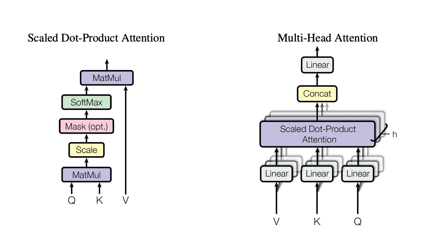
The raw score is divided by sqrt(d_k), the square root of the key-vector width. With large vectors, many products are added together, so scores can grow too large. Dividing keeps them in a range where softmax can learn without becoming immediately extreme.
After scores become percentages, the model multiplies each value vector by its percentage and adds the vectors. This weighted sum is the token's new context vector. A 50% weight means that value contributes much more than a value with a 5% weight.
Experiment in Playground 5: choose a different query token. Read each scaled score, its percentage, and the final context vector. Confirm that all percentages total approximately 100%.
Playground 5
Scaled Dot-Product Attention
Pick a query token. Its query scores every key; softmax turns scores into weights; the weighted values become a context-aware output.
Formula: Attention(Q,K,V) = softmax(QK^T / sqrt(d_k))V. Every percentage above participates in the weighted sum shown as the context vector.
5. Softmax turns scores into usable weights
Attention scores may be negative, positive, tiny, or large. Softmax converts them into positive weights that add to one. In plain language: exponentiate every score, then divide each result by the total. A larger score gets a larger share, but every token can still receive some weight.
The formula p_i = exp(s_i) / sum(exp(s_j)) says thatp_i is the percentage for score s_i. The denominator is the same for all tokens, which is why the final percentages sum to 100%.
Temperature provides another way to control sharpness. A low temperature exaggerates differences and makes one choice dominate. A high temperature flattens the distribution. Temperature is common during output sampling; this playground also uses it to make the softmax behavior easy to see.
Experiment in Playground 6: first change onlyd_k, then change only temperature. Find settings that make one token dominate, and settings that make the weights more even. Compare raw scores with scaled scores.
Playground 6
From Similarity Scores To Probabilities
Change the key dimension and temperature. Scaling controls exploding dot products; temperature controls how concentrated the distribution is.
| Key token | q dot k | scaled score | softmax weight |
|---|---|---|---|
| Ninja | 1.10 | 0.550 | |
| moved | 1.60 | 0.800 | |
| the | 0.40 | 0.200 | |
| plant | 2.20 | 1.100 | |
| near | 0.80 | 0.400 | |
| the | 0.30 | 0.150 | |
| window | 1.50 | 0.750 | |
| because | 0.70 | 0.350 | |
| it | 2.40 | 1.200 | |
| needed | 1.90 | 0.950 | |
| more | 0.90 | 0.450 | |
| sunlight | 1.70 | 0.850 | |
| . | 0.20 | 0.100 |
s_i = (q dot k_i) / sqrt(d_k)p_i = exp(s_i / T) / sum_j exp(s_j / T)6. Multiple heads can notice different relationships
One attention head produces one pattern of information flow. That can be restrictive: a sentence may simultaneously contain local grammar, a subject-action relationship, and a distant reference. Multi-head attention gives the model several independent sets of Q, K, and V projections.
Each head works in a smaller feature space and can learn a different pattern. Their output vectors are concatenated, meaning placed next to one another, and a final matrix W_O mixes them back into one d_model-wide vector.
Experiment in Playground 7: switch among all three heads. Find the local verb relationship, the link from it back to plant, and the need for sunlight. Then compare each pattern with the displayed mean. The note below the playground explains the real concatenation step.
Playground 7
Why Multi-Head Attention?
Switch heads to see different relationships. The right side averages these toy attention patterns only so they are easy to compare.
Head 1: local syntax
Ninja (2%)moved (3%)the (2%)plant (3%)near (3%)the (2%)window (4%)because (6%)it (18%)needed (42%)more (7%)sunlight (7%). (1%)Mean pattern for comparison
Ninja (2%)moved (4%)the (2%)plant (21%)near (3%)the (2%)window (7%)because (5%)it (11%)needed (21%)more (9%)sunlight (13%). (1%)Formula: MultiHead(Q,K,V) = Concat(head_1, ..., head_h)W_O, where each head_i has its own learned projections. A real Transformer does not average attention maps: each map mixes value vectors, then those head output vectors are concatenated and projected.
7. Attention lives inside a repeated block
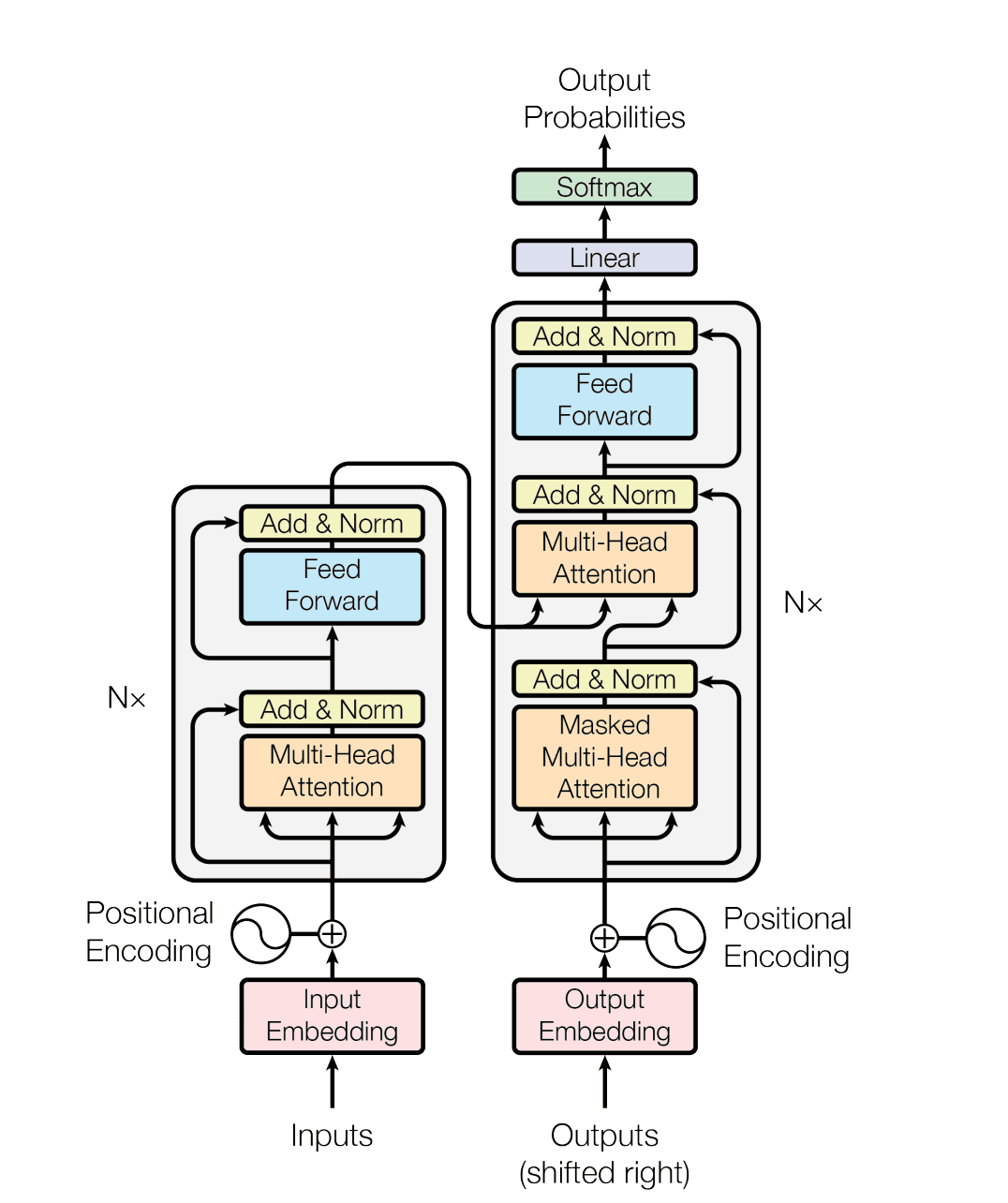
A Transformer is not one attention calculation. It stacks blocks. In an encoder block, multi-head attention first mixes information between token positions. A feed-forward network then transforms each position. Residual connections and normalization surround these operations.
Early layers may capture simple local patterns. Later layers receive already contextualized vectors and can compose richer behavior. Every layer preserves the sequence length and d_modelwidth, making blocks easy to repeat.
Experiment in Playground 8: select the six stages in order. For each stage, ask whether it mixes tokens with other positions, transforms one position, or protects the existing signal.
Playground 8
Inside One Encoder Block
Select each stage. The architecture repeats this pattern, allowing representations to become progressively more contextual.
Multi-head attention: Each token gathers useful context through several attention heads.
8. Residual paths preserve information
A sublayer should improve a representation without having to rebuild it from scratch. A residual connection computesy = x + Sublayer(x). The original vector xhas a direct route forward, while the sublayer contributes an update.
Layer normalization then looks across one token's features. It subtracts their mean and divides by their standard deviation. This produces a more controlled feature scale. Real LayerNorm also learns a scale and offset after normalization.
In (y_i - mean) / sqrt(variance + epsilon), epsilon is a tiny safety number that prevents division by zero. Mean describes the center; variance describes how spread out the values are.
Experiment in Playground 9: set the sublayer contribution to zero, then increase it gradually. Compare the original vector, residual sum, mean, variance, and normalized output.
Playground 9
Residual Paths And Layer Normalization
Scale the sublayer update. The shortcut preserves the original vector; layer normalization then recenters and rescales its features.
y = x + Sublayer(x)LayerNorm(y_i) = (y_i - mean) / sqrt(variance + epsilon)Current mean: 0.625; variance: 0.077. Learnable scale and bias are omitted here to keep the normalization visible.
9. The feed-forward network thinks per token
Attention moves information between token positions. The feed-forward network, or FFN, performs a nonlinear transformation on each position separately. The same FFN weights are reused for every position in the sequence.
The first matrix expands the vector into a larger hidden dimension. An activation function bends the numerical space, allowing behavior that stacked linear operations alone cannot express. A second matrix projects the hidden vector back to d_model.
ReLU replaces negative values with zero. GELU changes them smoothly instead of making a hard cut. The original Transformer used ReLU; GELU is common in later models.
Experiment in Playground 10: switch between ReLU and GELU. Follow the same vector through expansion, activation, and projection. Pay special attention to negative hidden values.
Playground 10
The Position-Wise Feed-Forward Network
Attention mixes information across positions. The feed-forward network then transforms each position independently using the same weights.
Formula: FFN(x) = activation(xW_1 + b_1)W_2 + b_2. The hidden dimension expands, applies a nonlinear transformation, then projects back to d_model.
10. A decoder must not look at future answers
When generating the French translation, the decoder should predict the next French token from target tokens already available. During training the complete correct translation exists in memory, so an unrestricted attention operation could cheat by reading future target tokens.
A causal mask adds zero to allowed scores and negative infinity to future scores. Softmax turns exp(-infinity) into zero, so future positions receive no attention. Each target position can see itself and its past, never its future.
Experiment in Playground 11: move the decoder query through the shifted French decoder input. At position zero,<BOS> predicts Ninja. At later positions, watch future input tokens remain blocked while the label names the separate token being predicted.
Playground 11
Causal Masking the French Target
The decoder receives a shifted target: it starts with <BOS> and never receives the token it must predict at that same position. Pick a position below; tokens to its right receive zero attention.
Mask rule: M(i,j) = 0 when j <= i, otherwise -infinity. Shifting prevents the current answer from appearing in the input; the mask prevents future answers from leaking backward. Training can still process every target position in parallel.
11. Encoder and decoder have different jobs
The encoder reads the complete English source sentence, Ninja moved the plant near the window because it needed more sunlight, and builds contextual representations for all source tokens. Its self-attention is not causal because the whole input is already known.
The decoder first uses masked self-attention on the target prefix. It then performs cross-attention: decoder states provide queries, while encoder outputs provide keys and values. This lets the decoder ask the source sentence for information needed at the current output position.
When the decoder is ready to produce plante, its query can assign strong weight to the English representation for plant. Later, producing parce qu’elle avait besoin de plus de soleildepends on the source clause because it needed more sunlightand on resolving it to plant rather than the nearer window.
Experiment in Playground 12: step through source encoding, French target-prefix reading, cross-attention, and French vocabulary prediction. At each step, identify where Q, K, and V originate.
Playground 12
Encoder Memory Meets Decoder Queries
Walk from the English source to the French translation one stage at a time. Cross-attention is the bridge that lets French target generation consult the English source sentence.
Encode English source
All English source tokens attend to one another and become contextual memory.
Ninja | moved | the | plant | near | the | window | because | it | needed | more | sunlight12. Decoding predicts one token at a time
The decoder's final hidden vector is projected to one number for every vocabulary token. These numbers are called logits. Softmax turns logits into next-token probabilities. In our running translation example, those candidates come from the French vocabulary.
Greedy decoding chooses the largest probability. Sampling draws from the distribution, allowing less likely choices. Whichever token is selected becomes part of the next input prefix, and the process repeats until an end token such as <EOS> is chosen.
Experiment in Playground 13: first choose the most likely French token at every step to produce Ninja a déplacé la plante près de la fenêtre parce qu’elle avait besoin de plus de soleil. Reset and choose alternatives to build a different toy prefix. The candidate lists are scripted for learning; a real decoder would recalculate later probabilities from the entire chosen prefix.
Playground 13
Generate the French Translation One Token At A Time
The English source remains Ninja moved the plant near the window because it needed more sunlight. Choose one French candidate at each step. It becomes part of the next decoder input, so generation is sequential at inference time.
Pipeline: hidden state -> vocabulary logits -> softmax -> token. Greedy decoding picks the largest probability; sampling can choose other candidates to increase variation. These candidate lists are scripted teaching examples, not probabilities recalculated by a live model; the omitted vocabulary holds the remaining probability mass.
13. Training rewards probability on the correct token
During supervised translation training, the correct next French token is known. The model's probability for that token is converted into cross-entropy loss: L = -log(p_correct). If the correct probability is near one, the loss is near zero. If it is near zero, the loss becomes large.
Gradient descent measures how each parameter influenced this loss and nudges millions or billions of parameters in a direction that should reduce future loss. Teacher forcing supplies the real previous token at every training position, so masked target positions can be scored in parallel.
Experiment in Playground 14: move the correct-token probability from 1% toward 99%. Notice that loss falls quickly at first and approaches zero, rather than decreasing in a straight line.
Playground 14
How The Model Learns A Better Prediction
Given the English source and French prefix <BOS> Ninja a, the correct next target token is déplacé. Move its assigned probability. Cross-entropy heavily penalizes confident wrong answers and approaches zero as the correct-token probability approaches one.
Formula for one target: L = -log p(correct token). During teacher forcing, the decoder receives the real previous target token, and this loss is accumulated across target positions.
14. Parallel computation still has a quadratic cost
Attention for many tokens can be expressed as matrix operations, which GPUs can perform in parallel. That is a major advantage over architectures that must finish one sequence step before starting the next during training.
Parallel does not mean free. With n tokens, there aren queries and n keys. Every query compares with every key, producing n x n = n squared scores. If length doubles from 8 to 16, cells increase from 64 to 256: four times as many.
This quadratic matrix is one reason long contexts consume substantial memory. Efficient-attention methods reduce the practical cost using locality, sparsity, compressed representations, or more memory-aware algorithms.
Experiment in Playground 15: try lengths 8, 16, 32, 64, and 128. Each time you double the length, verify that the exact score-cell count becomes four times larger.
Playground 15
The Quadratic Attention Tradeoff
Increase sequence length. Every query compares with every key, so doubling the token count creates four times as many score cells.
n x n = 8 x 8Full attention uses O(n^2) score memory and work per head. The preview is capped at 16 x 16 cells, but the count remains exact. Efficient-attention variants reduce this cost through sparsity, locality, compression, or kernel tricks.
15. From a Transformer to a modern chatbot
The original Transformer in the paper used an encoder to read a source sequence and a decoder to produce a target sequence. A common text-generation core in modern conversational LLMs uses a decoder-only Transformer. Instead of keeping an English sentence and French translation in two separate stacks, it places the available conversation into one ordered token sequence and predicts what should come next.
A chat interface may look like separate message bubbles, but the model receives a serialized sequence containing special boundaries for the system instruction, user messages, assistant messages, tool results, and other supplied context. Causal attention lets every position read earlier tokens while blocking later ones. The hidden state at the final position is projected into one logit for every vocabulary token.
Turn instructions and conversation messages into token IDs.
Use the causal Transformer to interpret the available context.
Produce one logit for every token in the vocabulary.
Use softmax to turn logits into a next-token distribution.
Choose one candidate and append it to the conversation.
Continue until a stop token or generation limit is reached.
This small repeated operation can produce a long answer because each chosen token changes the context for the next pass. The model does not merely match the last word: causal self-attention can use the whole available context window. Implementations commonly cache the earlier tokens' key and value vectors, called a KV cache, so generation does not need to rebuild all of that attention state from scratch after every token.
Pretraining on next-token prediction teaches language patterns and broad capabilities. Post-training then teaches the model to follow instructions, behave conversationally, and better reflect human preferences. Products such as ChatGPT and Gemini add a larger system around the model, which may include multimodal input processing, safety checks, retrieval, memory, and tool calls. Those additions provide new context or actions; text generation still proceeds by repeatedly selecting output tokens from the model's distribution.
Experiment in Playground 16: generate the answer one token at a time. Before each click, inspect the logits and probabilities. Change temperature and observe that the candidate distribution changes, then watch every selected token become part of the context used for the next prediction.
Further reading: the GPT-4 Technical Report describes next-token pretraining, while the Gemini 1.0 Technical Report describes a family built on Transformer decoders. Exact production architectures and surrounding systems vary by model and version.
Playground 16
Run A Chatbot's Next-Token Loop
This tiny decoder has already received the system instruction, user message, and source sentence as one context sequence. Generate the assistant reply one token at a time and watch the context grow.
- 1Read context
- 2Produce logits
- 3Apply softmax
- 4Select token
- 5Append and repeat
context tokens = prompt tokens + 0 generatedThelogit 3.470%Alogit 2.017%Becauselogit 1.28%Itlogit 0.85%The probabilities are a transparent toy example. A real LLM computes logits across its full vocabulary after every appended token. Lower temperature sharpens this distribution; higher temperature flattens it. Greedy decoding still selects the largest probability.
Nuances worth remembering
- Attention weights are routing signals: they show how values are mixed in one head and layer, but are not a complete explanation of model reasoning.
- Tokenization affects the sequence: the model predicts vocabulary pieces, not necessarily whole words.
- Position is a design choice: the original paper used fixed sinusoids; modern systems may use learned, relative, or rotary position methods.
- Training and inference differ: masked training can score known target positions together, while autoregressive inference must select each next token before continuing.
- One playground is one layer-level view: real model behavior is composed across many heads, residual updates, nonlinear transformations, and repeated blocks.
The complete mental model
- Tokenize text and look up embeddings.
- Add position information.
- Project each representation into Q, K, and V.
- Use scaled dot products and softmax to route information.
- Run several heads, then combine their outputs.
- Use residuals, normalization, and an FFN inside each block.
- Mask future target tokens inside the decoder.
- Use cross-attention to read encoder memory.
- Predict one next token and train using cross-entropy loss.
- Append the selected token and repeat until generation stops.