Computer vision systems
ImageNet Classification with Deep Convolutional Neural Networks
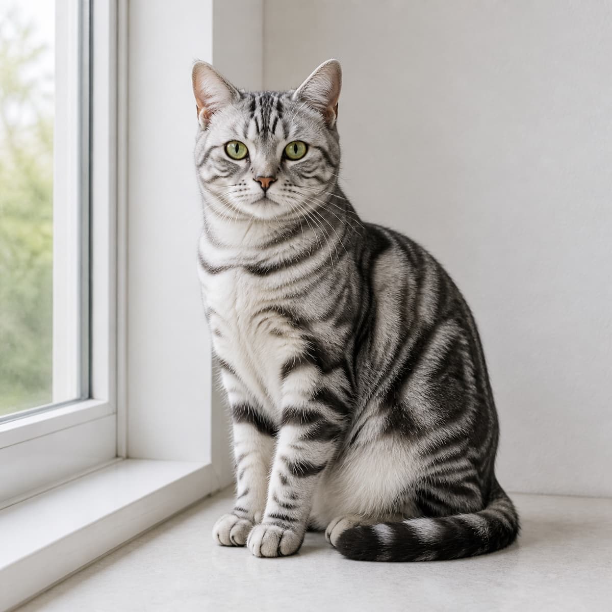
Running example
Can AlexNet recognize this silver tabby?
We will carry this exact image from raw pixels to the final class ranking. The goal is to see what each stage contributes, not just memorize a stack of layer names.- PixelsColor and brightness values enter the network.
- EdgesEarly filters respond to ears, whiskers, stripes, and the window frame.
- PartsDeeper layers combine edges into eyes, fur texture, paws, and a face.
- ClassThe classifier ranks tabby-cat labels above unrelated objects.
The 2012 turning point
Image classification asks a model to receive pixels and choose a label such as tabby cat, school bus, or volcano. The same object can move, rotate, change scale, appear under different light, or be partly hidden. A useful model must recognize the object rather than memorize one arrangement of pixels.
In 2012, Alex Krizhevsky, Ilya Sutskever, and Geoffrey Hinton trained the network now called AlexNet on roughly 1.2 million ImageNet training images spanning 1,000 classes. The model combined five convolutional layers, three fully connected layers, ReLU, overlapping max pooling, data augmentation, dropout, and a highly optimized two-GPU implementation.
Its ILSVRC-2012 entry reached 15.3% top-5 test error, compared with 26.2% for the second-best entry. The important lesson was larger than one leaderboard result: with enough labeled data, computation, regularization, and a deep architecture, a neural network could learn useful visual features directly from pixels.
Primary source: Krizhevsky, Sutskever, and Hinton, ImageNet Classification with Deep Convolutional Neural Networks. Dataset context: the ImageNet Large Scale Visual Recognition Challenge.
1. Convolution learns local visual detectors
A normal dense layer would connect every input pixel to every output unit. That ignores an important fact about images: nearby pixels are strongly related, and the same small pattern can appear anywhere. A convolutional layer instead learns a small grid of weights called a kernel or filter.
The filter slides across the image. At each position it multiplies its weights by the pixels under it and adds the products. This is a dot product. Repeating it at every position creates a feature mapthat answers: “where did this pattern occur, and how strongly?”
The same filter weights are reused at every location. This is weight sharing. It dramatically reduces parameter count and lets one learned edge detector respond on the left, center, or right of an image. Deeper layers apply new filters to earlier feature maps, composing edges into textures, parts, and objects.
Our cat: one early filter may activate on the bright whiskers against dark fur, another on the ear boundary, and another on the vertical edge of the window. It does not yet know that any of these pixels belong to a cat.
Experiment in Playground 1: choose the edge, vertical edge, and blur kernels. Move the receptive field over the bright shape. Read the nine products and verify that their sum becomes one output activation.
Playground 1
Slide A Learned Filter Across Pixels
Move the 3 x 3 receptive field, choose a filter, and inspect every multiply-and-add operation that creates one output activation.Cat image to simplified pixel patch
The 5 x 5 values below are a deliberately simplified, binary zoom into a high-contrast region near the cat's face.
Edge detector kernel
One dot product
0 x -1.00 = 0.001 x -1.00 = -1.001 x -1.00 = -1.001 x -1.00 = -1.001 x 8.00 = 8.001 x -1.00 = -1.001 x -1.00 = -1.001 x -1.00 = -1.000 x -1.00 = 0.00During training, the network learns useful kernel values. One kernel produces one feature map; many kernels learn different patterns such as oriented edges, colors, textures, and eventually object parts.
2. Stride, padding, channels, and output shape
Stride is how far a filter moves between positions. A large stride produces a smaller map because it samples fewer locations. Padding adds pixels around the border so filters can be centered near the original edge. Kernel size controls how large a local neighborhood one output reads.
For one spatial dimension, the output width isfloor((input + 2 x padding - kernel) / stride) + 1. The floor matters: if the last step would place part of the kernel outside the padded input, that position is discarded.
Images and feature maps also have channels. One RGB image has three. A convolution filter spans every channel it is connected to, then writes one output map. AlexNet Conv1 used 96 filters, so it produced 96 output channels.
Our cat: the photograph is resized and cropped into a 227 x 227 x 3 tensor for this walkthrough. Conv1 turns that single RGB image into 96 different 55 x 55 maps, each looking for a different low-level pattern.
Experiment in Playground 2:begin with AlexNet's 227, 11, 4, 0 settings. Then reduce stride, add padding, or enlarge the kernel. Predict whether the feature map will grow or shrink before reading the result.
Playground 2
Calculate A Feature Map's Shape
Adjust input size, kernel, stride, and padding. The AlexNet defaults below reproduce its first 55 x 55 feature map.floor((227 + 2 x 0 - 11) / 4) + 155 x 55Every final stride lands exactly.A filter also spans every input channel. AlexNet's first filters are 11 x 11 x 3 because RGB images have three channels, but each filter still writes one two-dimensional feature map.
3. ReLU made deep training practical
After a convolution or dense layer calculates a weighted sum, an activation function adds nonlinearity. Without nonlinear activations, stacking many layers would still collapse into one linear transformation and could not represent complex visual decisions.
AlexNet used ReLU(x) = max(0, x). Negative inputs become zero; positive inputs pass through unchanged. Earlier networks often used tanh or sigmoid, whose outputs flatten near their extremes. Gradients through those saturated regions become small, slowing learning in deep networks.
The paper reported that its ReLU network reached a particular training-error level about six times faster than an equivalent tanh network. ReLU did not make learning effortless, but it removed an important optimization bottleneck.
Our cat: a positive response from a whisker or stripe detector survives ReLU. A negative response becomes zero, leaving a sparse map of locations where that learned pattern was found.
Experiment in Playground 3:sweep the input from -6 to +6. Notice tanh and sigmoid approaching flat ceilings while ReLU remains linear for positive inputs. Also notice ReLU's zero output for every negative value.
Playground 3
Compare ReLU With Saturating Activations
Move one pre-activation value and compare the output curves. ReLU preserves a straight gradient for positive inputs.ReLU is not bounded above, so positive activations do not squeeze toward a flat ceiling. AlexNet reported reaching a target training error much faster with ReLU than with an otherwise equivalent tanh network.
4. Pooling compresses nearby responses
Max pooling moves a small window over each feature map and keeps only its largest activation. This reduces width and height, lowers later computation, and gives the representation some tolerance to small shifts. If a strong edge moves by one pixel but remains inside the same pooling neighborhood, the pooled output can stay unchanged.
AlexNet used overlapping pooling: a 3 x 3 window with stride 2. Because the window is larger than the stride, neighboring windows share pixels. Pooling does discard exact location and weaker responses, so it is a tradeoff rather than a universally harmless operation.
Our cat:if a strong ear-edge response moves a pixel because the crop shifts slightly, max pooling can retain nearly the same evidence while reducing the feature map's size.
Experiment in Playground 4: move between the four pooling windows. Compare max pooling with the average of the same values and find activations that belong to two neighboring windows.
Playground 4
See Overlapping Max Pooling
AlexNet used a 3 x 3 pooling window with stride 2. Neighboring windows overlap by one row or column and retain the strongest activation.1, 2, 1, 0, 5, 2, 2, 1, 45. AlexNet's complete architecture
AlexNet progressively trades spatial resolution for channel depth. The early 55 x 55 maps preserve location. Later 13 x 13 maps carry hundreds of learned channels. After the final pool, a 6 x 6 x 256 tensor is flattened into 9,216 numbers and passed through two 4,096 unit dense layers before the 1,000-class output.
The convolutional layers learn reusable spatial features, but most parameters sit in the dense classifier. FC6 alone contains about 37.7 million weights and biases. Across the architecture, the usual calculation gives roughly 61 million parameters, close to the paper's rounded 60 million figure.
AlexNet also used local response normalization (LRN)after Conv1 and Conv2. It encouraged competition between nearby channels. Batch normalization and other techniques later made LRN uncommon, but it belongs in an accurate historical description.
Our cat: early layers represent edges and color transitions. Middle layers can combine them into striped fur, eyes, ears, and paws. Later layers integrate those parts into a cat-shaped representation before the dense classifier sees it.
Experiment in Playground 5:walk from Input through FC8. Track shrinking spatial dimensions, growing channels, and the cumulative parameter count. Compare Conv5 with FC6 to see why dense layers dominate AlexNet's parameter budget.
Playground 5
Walk Through AlexNet Layer By Layer
Select a stage to track tensor shape, operation, and parameter count. Notice where most of the parameters actually live.Conv1
96 filters, 11 x 11, stride 4. Followed by ReLU, LRN, and pooling.
6. Data augmentation teaches invariance
Sixty million parameters can memorize a training set. AlexNet fought this by generating altered training views without changing the label. Images were resized to a common 256 x 256 canvas, then random 224 x 224 crops and horizontal reflections were sampled during training.
The paper also added multiples of ImageNet's principal RGB color directions. In simpler language, it shifted image colors along the major ways color varied in the dataset. The object identity stayed the same, so the model had to become less dependent on one crop, reflection, or lighting balance.
Our cat: a left-shifted crop, a horizontal reflection, or a modest color change is still the same tabby. The label must not change when these nuisance details change.
Experiment in Playground 6: move the crop, reflect the pixel image, and change its intensity. Observe that the pixel arrangement changes while the semantic label remains fixed.
Playground 6
Create New Training Views Without New Labels
Shift the crop, reflect it, and perturb its color channel. Every view keeps the same class label while changing the pixels the model sees.The pixels and framing changed, but the semantic class did not. The brightness control is a simplified stand-in for AlexNet's RGB color augmentation.
7. Dropout prevents hidden units from relying on one team
During dropout training, each participating hidden unit is randomly set to zero with some probability. A feature cannot assume that one particular partner will always be present, so useful evidence must be distributed across many subnetworks.
AlexNet applied 50% dropout in FC6 and FC7. At test time all units participate, but their outgoing contribution is scaled to match the average training-time signal. The paper notes that dropout roughly doubled the iterations needed for convergence while substantially reducing overfitting.
Our cat: the classifier should not depend on one hidden unit that happens to recognize stripes. During training, dropout forces it to also use evidence such as ears, eyes, paws, face shape, and body outline.
Experiment in Playground 7: draw several masks at 50%, then compare 20% and 80%. Watch individual units disappear while the test-time expected scale remains deterministic.
Playground 7
Break Co-Adaptation With Dropout
Randomly silence hidden units during training. The original AlexNet used a 50% dropout rate in its first two fully connected layers.AlexNet's original convention kept surviving activations unchanged during training, then multiplied outgoing weights by the keep probability at test time. Many current libraries instead scale survivors during training, producing the same expectation.
8. The training recipe mattered too
Architecture alone did not produce the result. AlexNet trained with stochastic gradient descent using mini-batches of 128 examples, momentum 0.9, and weight decay 0.0005. The learning rate began at 0.01 and was divided by ten when validation error stopped improving.
The authors trained for about 90 passes through the data over five to six days on two 3 GB NVIDIA GTX 580 GPUs. The network was split because one GPU could not hold it. Conv2, Conv4, and Conv5 used grouped connectivity within a GPU, while Conv3 communicated across the split. Modern grouped convolution APIs preserve this historical architecture detail.
This is a systems lesson as much as a machine-learning lesson: AlexNet was a co-design of model, optimization, regularization, data pipeline, and GPU implementation.
9. Softmax, top-1, and top-5 classification
FC8 emits 1,000 raw scores called logits. Softmax exponentiates and normalizes those scores into a probability distribution. The largest probability is the model's top-1 prediction; the five largest form its top-5 set.
Top-1 error counts an image wrong unless the true label is ranked first. Top-5 error counts it correct when the true label appears anywhere among the first five. Top-5 was useful for ImageNet because fine-grained categories can be visually similar and some images plausibly contain multiple objects.
On the LSVRC-2010 test set, the paper reports 37.5% top-1 error and 17.0% top-5 error for its model. Its separate ILSVRC-2012 competition entry achieved the headline 15.3% top-5 test error. Keeping those evaluation settings separate avoids mixing two different results.
Our cat: the final logits might rank tiger cat, Egyptian cat, tabby cat, lynx, and Persian cat above laptop or banana. If the target label is tabby cat, that result is wrong under top-1 but still correct under top-5.
Experiment in Playground 8: keep tabby cat as the ground truth and compare top-1 with top-5. Then choose laptop or banana. Change temperature and verify that confidence changes while rank order does not.
Playground 8
Turn 1,000 Logits Into Top-1 And Top-5 Results
This small vocabulary stands in for ImageNet's 1,000 classes. Choose the ground-truth label and inspect both evaluation metrics.Temperature changes confidence but not rank order when every logit is divided by the same positive number. ImageNet competition results often reported top-5 error because many categories are visually similar.
10. What later networks kept and changed
- Kept: learned convolutions, ReLU-like nonlinearities, augmentation, GPU training, and end-to-end supervised learning.
- Changed: later CNNs often use smaller kernels, deeper stacks, batch normalization, residual connections, and global average pooling instead of enormous dense layers.
- Mostly retired: LRN and the two-GPU split were solutions to the optimization ideas and hardware limits of their era.
- Still essential: the result depends on a complete training system, not an architecture diagram in isolation.
AlexNet was not the first convolutional neural network, and many of its individual ingredients already existed. Its lasting importance is that it assembled those ideas at ImageNet scale and demonstrated a decisive practical result. It made deep learned visual features the new baseline for computer vision.
The complete mental model
- A filter reuses local weights across the image.
- Each filter produces one feature map.
- Stride and pooling reduce spatial size.
- More channels represent more learned visual patterns.
- ReLU keeps useful positive gradients flowing.
- Augmentation and dropout reduce overfitting.
- Dense layers convert visual features into class logits.
- Softmax ranks the 1,000 ImageNet classes.